Spline Overview

Why Use Cubic Splines?

Some applications require that the motion controller move between a number of positions that vary for each sequence of moves. An example of this is curve sawing. In this application a cant (a section of a log) is scanned, and an optimizing computer determines the best path for the saws through the cant. The motion controller then must follow this smooth path through the cant.

The most basic way to follow this curve would be to select various positions along the cant and calculate where the saws need to be at each length on the cant. Then the programmable controller could give commands to go to the various positions. The problem with using this method is that for each Go (G) command, the motion controller will ramp up to a constant velocity, and then ramp down to a stop for each point. This would not give a smooth curve through the entire cant.

Another method would be to carefully control the speed of a move to the extend or retract limit so that the saws follow the curve. The problem with this method is that a large number of calculations must be done in the programmable controller.

To greatly simplify the work required by the programmable controller and also provide smooth moves between points along a curve, the RMC has been equipped with cubic splines. When using cubic splines, the programmable controller needs only to send the positions where the axis should be located at various times along the curve. The RMC takes care of creating a curve that is smooth for position and velocity and continuous for acceleration.

Basic Vocabulary

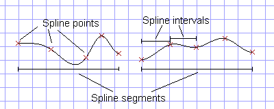
Refer to these example splines for the following definitions.

Spline Point:

The user defines several spline points for a single curve. In the example shown above, the X's mark the points set by the user. The horizontal direction in this graph is time and the vertical direction is the axis position.

Spline Interval:

The user controls the number of master units between the spline points. Master units can be any of three quantities:

• Master Axis Position Units. If the curve is followed with a master axis selected, then each master unit will correspond to one position unit on the master axis. See the Follow Spline (f) and Follow Spline Relative commands for details on following a spline with a master axis. This is the most common way of following a spline.

• Time. If the curve is followed without a master axis selected, and no Digital I/O module counter is enabled (see Using Counters), then each master unit will correspond to 1/1024th of a second.

• Counter Ticks. If the curve is followed without a master axis selected, and a Digital I/O module counter is enabled (see Using Counters), then each master unit correlates to one counter tick. This method is largely historical. It is usually better to use the Master Axis Position Units as master units, but this method was introduced before the RMC's Quadrature module was available.

The interval between spline points cannot be greater than 65,535 master units or less than 10 units.

Spline Segment:

The RMC can hold several spline curves in its memory at a time; each is called a segment. There is no exact limit for how many points can be in a segment, but there is a limit for the total number of points among all segments in the motion controller. This limit is 1023 points per axis on a 2-axis RMC, 511 points per axis on a 3- to 4-axis RMC, and 255 points per axis on RMCs with five or more axes.

Standard vs. Enhanced Splines

The RMC supports two types of curves: Standard and Enhanced. Each is described below.

Standard Curves

Standard curves were introduced with RMC CPU firmware dated 19971204. This gave the RMC the capability of following curves defined by cubic splines. The user defines the position and time of each point in the curve. The velocities of the endpoints are fixed at zero (0). The velocities of all other points and accelerations of all points are computed by the RMC to find the smoothest curve through all points.

There are several deficiencies with Standard curves:

• Because the accelerations are computed at the endpoints, it is likely that they will be non-zero and therefore result in an acceleration discontinuity and relatively high jerk at each endpoint.

• It is difficult to accurately approximate a linear segment.

• It is difficult to set and maintain a given velocity at a given point.

• The velocities at the endpoints could not be changed from zero (0).

These issues prompted the introduction of Enhanced curves.

Enhanced Curves

Enhanced curves were introduced with RMC CPU firmware dated 20010208. They greatly enhance the capabilities of the RMC in following an arbitrary curve, and further enhance the smoothness of the curve.

The following items are introduced with enhanced curves:

• The accelerations at the endpoints of a curve are always zero (0). Therefore, there is no acceleration discontinuity and therefore much lower jerk at the end points. The acceleration is continuous over the entire curve, even with the additional features listed below.

• Segments can be easily designated as linear segments, which makes them exactly linear. This greatly simplifies camming and flying cut-off applications.

• Any point, including the endpoints, can have its velocity set to a specific value. This, too, simplifies camming and flying cut-off applications.

• Curves can be set up to auto-repeat, meaning that the curve restarts automatically when it reaches its end. See Auto Repeat Curves for details.

The drawback of Enhanced curves is that they can currently only be downloaded to the RMC through RMCWin's Curve Tool, and not from a Programmable Controller through communication modules such as Ethernet, PROFIBUS, and Modbus Plus. See Curve Tool Overview for details on the Curve Tool.

You should always use Enhanced curves unless you are running firmware prior to 20010208 and do not wish to upgrade, or you need to download curves through the communication module.

What If I Don't Want Zero Velocity at My Endpoints?

Each spline segment in a Standard curve will begin and end at zero velocity. This is desirable so that when a motion controller's axis is given the command to follow a spline curve, the axis does not instantly jerk to the new velocity. However, there are applications where the curve does not begin with zero velocity.

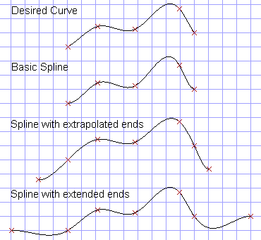
If the curve is downloaded from RMCWin, then you can switch to use an Enhanced curve which allows the velocity of each point to be set. However, if the curve is being downloaded over Ethernet, Modbus Plus, PROFIBUS or some other communication module, it is recommended that the user add one or more points to the beginning and end of the curve. The following curves demonstrate how this can be done:

The first curve is the actual curve that we want to match. The second curve is the one that would be generated by the RMC if no leading or trailing points were used. The velocities do not match well at the ends in this curve. In the third curve, one point is added to the front and one point is added to the end. In this curve, the endpoints were placed the same distance and time from the original endpoints as the second points from the ends. In the fourth curve, the new endpoints are added at the same position as the original endpoints, but are a fixed time from the original endpoints. This method works best when the time between the original and new endpoints are at least twice the distance between the original first and second points.

The best method to use depends on the application, and is not limited to the above methods.

Using Cubic Splines

There are three ways to get the points in a cubic spline into the RMC:

• Download curves from the Curve Tool. See Curve Tool Overview for details.

• Issue the commands described below over the communication module.

• Use the Spline Download Area. For a discussion of the tradeoffs between these three methods and further details on using the Spline Download Area, see Downloading Splines to the RMC.

Only the first method can generate Enhanced curves, the other two will generate Standard curves.

Using the Cubic Spline Commands

There are five commands that apply to cubic splines. Click on any of the command names below for further details on each:

Add Spline Point  This is used to add a point to the end of a new segment.

Set Spline Interval  This is used to control the time/counter ticks between points.

End Spline Segment  This is used to indicate the end of a segment and perform final calculations on the curve.

Clear Spline Segments  This is used to clear one or more segments from the motion controller's memory.

Follow Spline Segment  This causes the axis to follow a single spline segment. The motion controller updates the spline every millisecond. The axis must already be at the position of the first point for this command to succeed.

Follow Spline Relative  This causes the axis to follow a single spline segment relative to the current axis position. This command is similar to the Follow Spline (f) command but does not require the axis to be at the position of the first spline point.

In addition to these five commands, there are two other ways to download splines. They are described under Downloading Splines to the RMC. When using other methods of download splines—using the Spline Download Area and using RMCWin—the first three commands listed above are not used, but the final two still apply.

A Cubic Spline Example

Suppose that a cant (a section of a log) is scanned for a curve sawing application. For simplicity, we assume the cant was scanned at only seven points. We also assume that we're using a Sensor Digital I/O to keep track of the quadrature counter on the belt moving the cant. Therefore, we'll also assume that the cant was scanned at a uniform distance between readings of 200 quadrature counts.

Therefore, suppose the optimizer gave the following readings:

In this application it is not safe to assume that the saws should be at zero velocity at the ends of the cant. Therefore, we'll use one of the methods described above for getting non-zero velocities at the ends: we will add a point to the beginning and end of these sets of points. So the new data will look like this:

The optimizer must then send this spline segment to the motion controller. Assuming that the optimizer cannot use RMCWin to download the spline, there are two methods of doing this. The first is to use the Add Spline Point, Set Spline Interval, and End Spline Segment commands. The second is to use the Spline Download Area. An example of the steps required to do each is shown below:

Downloading with the Spline Download Area:

You should look over Downloading Splines to the RMC for details used in this example. To use the Spline Download Area for this example, you need only write two blocks of data to the RMC's Spline Download Area. First, you would write the following data to give the count and time intervals. Addresses are given in Modbus (RTU, TCP, and Plus) format. See Downloading Splines to the RMC for other communication module addressing formats.

Now that the RMC knows the number of points we will download and the intervals between these points, we can download the point positions:

Downloading with Add Spline Point, Set Spline Interval, and End Spline Segment Commands:

The following commands would be issued in order:

In this example, notice that the case of the Add Spline Point (X) command is toggled each time it is used. In order for the motion controller to process a command, it must detect that the command or command value has changed. Therefore, by toggling the case of the 'X' command, each point will be processed even if two points have the same value (as is the case with the last two points).

The following graph demonstrates what the loaded spline will look like, with the vertical gridlines being 100 counts apart and the horizontal gridlines being 1000 position units (1 inch) apart.

Next, suppose an electric eye in front of the saws detects when a cant is about to be cut. A cant will trigger this electric eye a fixed number of counts before it reaches the blades. In our example, this eye is 1000 counts in front of the saws. Because of the leading point added to the spline, our spline begins 400 counts before the cant itself, so we must delay 600 counts from the time the electric eye detects the beginning of the cant to the time that we begin following the spline.

The programmable controller can take care of this time delay, however it is also possible to process this input using the Input to Event and Event Step tables in the RMC. To do this, the output from the electric eye can be run into the motion controller's CPU input 0. CPU output 0 will then be run back to the programmable controller to indicate when the cut is completed. The entry in the Input to Event table for this input will hold the Event Step 1. The Event Step table would look something like this.

In the first step, we reset the output to the programmable controller and wait for the input from the electric eye to trigger. After this occurs, we move to step 2 and delay for 600 counts. After the delay, event step 3 will be executed, which issues an 'f' command that makes the motion controller begin following the spline. After the In Position bit of the STATUS word is set, then step 4 is executed. At this point the CPU output 0 is set high and held high for 20 milliseconds to let the programmable controller know that the cant has been cut. The sequence is then repeated.

Copyright (c) 1997-2015 by Delta Computer Systems, Inc.