Valve Linearization

Valve linearization refers to compensating for non-linear hydraulic valves.

Valve Types

Linear and non-linear refer to the flow versus command signal profile of a valve. Typically, Delta recommends using linear valves. Linear valves are nearly always of very high quality, provide excellent response and are very easy to set up. Very high-quality, non-linear valves may be useful in certain situations that require high flow together with very fine positioning or pressure accuracy.

Linear

Non-linear

The flow is proportional to the command signal input and does not require linearization.

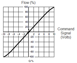
Notice that it is common for the flow profile to roll off as it approaches 100%. This is common, and the valve is still considered linear.

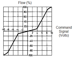
Single-knee

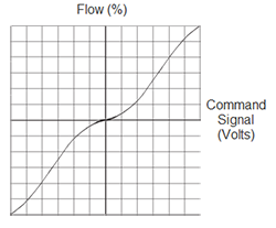
Curvilinear

The flow has a single sharp 'kink' and can be linearized via the Single-Point method.

These flow profiles can be linearized via curves.

Linearization Types

Valve linearization is applied only when the axis is in closed loop control. The RMC supports valve linearization via two methods:

Single-Point
Used only for valves with a single "knee" or "kink" in the flow versus command signal diagram
Curves
Used for valves with any flow diagram, especially curvilinear valves.

Single-Point Valve linearization

The RMC provides single-point valve linearization to compensate for valves with one sharp "knee" or "kink" in the flow versus command signal diagram, as shown above. The flow diagram is assumed to include the points (0,0), (-100,-100), and (100,100).

To Apply Single-Knee Valve Linearization:

In the Axis Tools, in the Axis Parameters Pane, on the All tab, expand the Output section.
In the Valve Linearization Type cell, choose Single-Point
Set the axis parameters as follows:

RMC75/150:

Knee Command Voltage: The input voltage value of the knee. This voltage can be obtained from the valve data sheet. For example, in the Single-Knee Valve diagram above, on the horizontal axis, the voltage is 4 volts.

Knee Flow Percentage: The flow percentage of the valve at the knee. This value can be obtained from the valve data sheet. For example, in the Single-Knee Valve diagram above, on the vertical axis, the flow percentage is 10%.

RMC200:

Knee Command Input: The input value of the knee. This percentage value can be obtained from the valve data sheet. For example, in the Single-Knee Valve diagram above, on the horizontal axis, the voltage of 4 volts would equal an input value of 40%.

Knee Flow Output: The flow percentage of the valve at the knee. This value can be obtained from the valve data sheet. For example, in the Single-Knee Valve diagram above, on the vertical axis, the flow percentage is 10%.
Download the changes and update Flash.

If the valve has an overlapped spool, the Output Deadband and Deadband Tolerance axis parameters can be used as normal.

Curve Valve linearization

Valve linearization via curves may be used to compensate for valves with any flow versus command signal diagram.

To Apply Valve Linearization via Curves:

Using the Curve Tool, create a curve for valve linearization. See Creating a Curve for Valve Linearization below.
You can also import existing valve linearization curves into the Curve Tool.
In the Axis Tools, in the Axis Parameters Pane, on the All tab, expand the Output section.
In the Valve Linearization Type cell, choose Curve.
In the Valve Linearization Curve ID cell, enter the number of the desired curve to use for linearization.
Download the changes and update Flash.

Creating a Curve for Valve Linearization

To create a curve for valve linearization, make a curve that matches the flow profile of the valve, with the x-axis being the input signal in percent, and the y-axis being the flow output in percent. For overlapped-spool valves, see CurveValve Linearization and Deadband below.

Most valve flow profiles are given as positive flows for both positive and negative x-values. The curve must have negative flows for negative x-values.

The curve must meet the following requirements:

Curve Properties:

Curve Type must be Valve Linearization.
Endpoint Behavior must be Natural Velocity.
Interpolation must be Linear or Cubic.

The first point must be (-100, -100).
The last point must be (100, 100).
The curve must contain the point (0,0).
The x-values must be within the range -100 and 100.
The y-values must be within the range -100 and 100, including the interpolated portions of the curve between points.
The curve must be positive monotonic. This means the curve is always increasing or flat. Any flat section, if present, should only be around the point (0,0). See Curve Valve Linearization and Deadband below.

Tip: If the y-values of the flow profile are in gpm or lpm, you will need to convert them to percent when creating the curve.

Example:

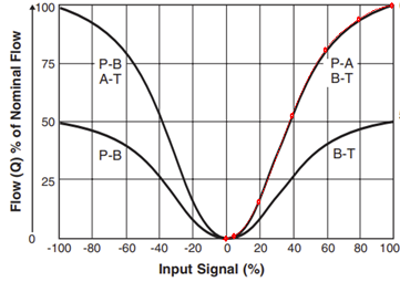
Consider profile E in this valve flow profile diagram:

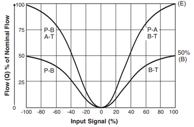
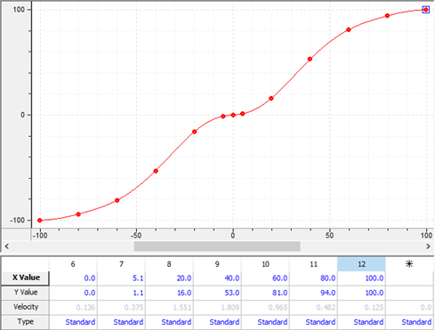
The following curve was created for this flow profile. Points were chosen at 20, 40, 60, and 80, plus an additional point close to zero (5.1, 1.1) so that the curve follows the profile accurately in that region. The negative values mirror the positive values.

One way to verify that the curve matches is to take a screen shot and overlay the curve on the flow profile using an image editing program:

Curve Valve Linearization and Deadband

Deadband refers to the range for an overlapped spool where the flow is zero until the command signal reaches a certain value.

If the valve has deadband, follow these steps for valve linearization via curves:

Create a curve that matches the valve flow profile and select that curve for the axis' valve linearization. See Creating a Valve Linearization Curve with Deadband below.
If the axis hunts when it is in position, you can mitigate it as follows:

Set the Output Deadband axis parameter to the deadband of the valve.
Set the Deadband Tolerance axis parameter to a small value. This will ratio the Output Deadband when the Actual Position is close to the Command Position to prevent hunting. The axis typically holds position within a tolerance of about half of the Deadband Tolerance.

Creating a Valve Linearization Curve with Deadband

A linearization curve for a valve with deadband must follow the requirements listed in Creating a Curve for Valve Linearization above. It can be especially challenging to create the flat spot around zero, since the curve tends to become non-monotonic.

To make a curve flat around zero:

For the two points next to zero on the x-axis (the points to the left and right of zero), set the y-values to zero.

If using a cubic interpolation:

For the point to the left of zero, and for the point at zero, in the spreadsheet editor, set the point type to Const Vel.
Or, in CurveProperties, you can set the Auto Constant Velocity Behavior to Enabled.

Tip: The actual deadband of the valve may vary from the profile given in the datasheet. You may need to manually determine the deadband of the valve and adjust the curve accordingly.

Example

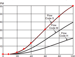
Consider profile S in this valve flow profile diagram:

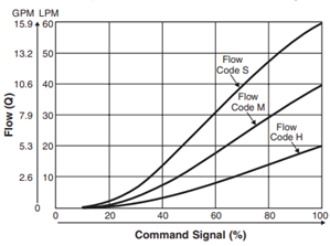
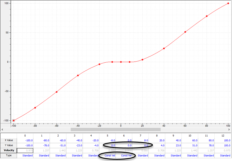
The curve below was created for this flow profile. Points were chosen at 8, 20, 30, 40, 60, and 80 so that the curve follows the profile accurately. The y-points were converted to percent. The negative values mirror the positive values.

Notice that the y-values for points 5, 6 and 7 are zero, and the Type for points 5 and 6 is Constant Velocity. The Constant Velocity type is necessary to maintain the monotonicity of the flat section of a cubic-interpolated curve.

Overlaying the curve on the flow profile using an image editing program shows that the curve closely follows the profile: