Feedback Linearization using Curves

This topic describes how to implement single-axis feedback linearization by using a curve to define the relationship between the transducer and the real measurement you need. For example, a curve can be used to linearize a transducer with as many points as you need. Or, consider a transducer mounted in a cylinder that drives a swing arm, but you actually need the position of the end of the arm. Given the machine geometry, a curve can be used to convert the transducer measurement to the position of the swing arm.

Another method of feedback linearization is via a mathematical formula, as described in Feedback Linearization Using a Mathematical Formula.

Tip: The Examples section of Delta's online forum includes a Feedback Linearization Using Curves example. You can use that example to help you get started.

Setting Up Feedback Linearization

Read the Custom Feedback topic before completing this procedure.

1. Determine Actual Measurement Versus Transducer Measurement

Determine the relationship of the desired true measurement to the transducer's measurement. This may be in the form of an equation, or measurements taken at a number of points throughout the transducer's measurement range.
Assemble the data as a table of data consisting of the desired true measurements and the transducer's measurements. If you have an equation, you can use a spreadsheet program such as Microsoft Excel to calculate points from the equation.

2. Create a Curve

Create a new curve in the Curve Tool.
In the curve data, enter the transducer's values in the x-axis. Enter the desired true measurements in the y-axis. If you have the data in a spreadsheet program such as Microsoft Excel, you can copy the data and paste it into the Curve Tool.
Make sure the x-values will cover the entire travel range of the physical feedback. If it does not, you may encounter a runtime error when you run the system.
In the curve properties, set the Endpoint Behavior to Natural-Velocity.
In the curve properties, set the Interpolation to either Cubic or Linear, as required by your application.

Note: It is important that the x-axis contains the transducer's values, and the y-axis contains the desired true measurements.

3. Define Custom Axis and Reference Axis

Define a control axis with the feedback type required (position, velocity, pressure, force, or acceleration). For the feedback source, choose Custom.
Create a reference axis for the feedback input to be used.
Configure the feedback parameters for the reference axis and verify that the transducer gives valid readings.
Set the Scale and Offset so that the reference axis provides correct values throughout the entire range.

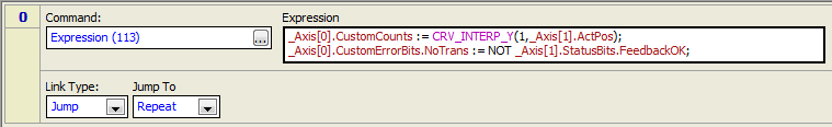
4. Use the Curve in the Custom Feedback User Program

Create a single-step user program with a Jump Link Type and a Repeat Jump To location.
Add an Expression (113) command.
In the expression, use the CRV_INTERP_Y function to get the curve's interpolated desired true value from the transducer's measurement.
Set the CustomErrorBits.NoTrans bit according to the state of the active feedback. This can be done by using the Feedback OK status bits of the reference axes.

5. Make Sure the User Program Always Runs

As described in more detail in the Custom Feedback topic, do the following:

Set the RMC to start in RUN mode.
Use a _FirstScan condition in the Program Triggers to start the user program when the RMC enters RUN mode.
Make sure the Task does not stop when an axis halts.

6. Tune the Axis

Tune the axis manually (auto-tuning does not work in RUN mode).